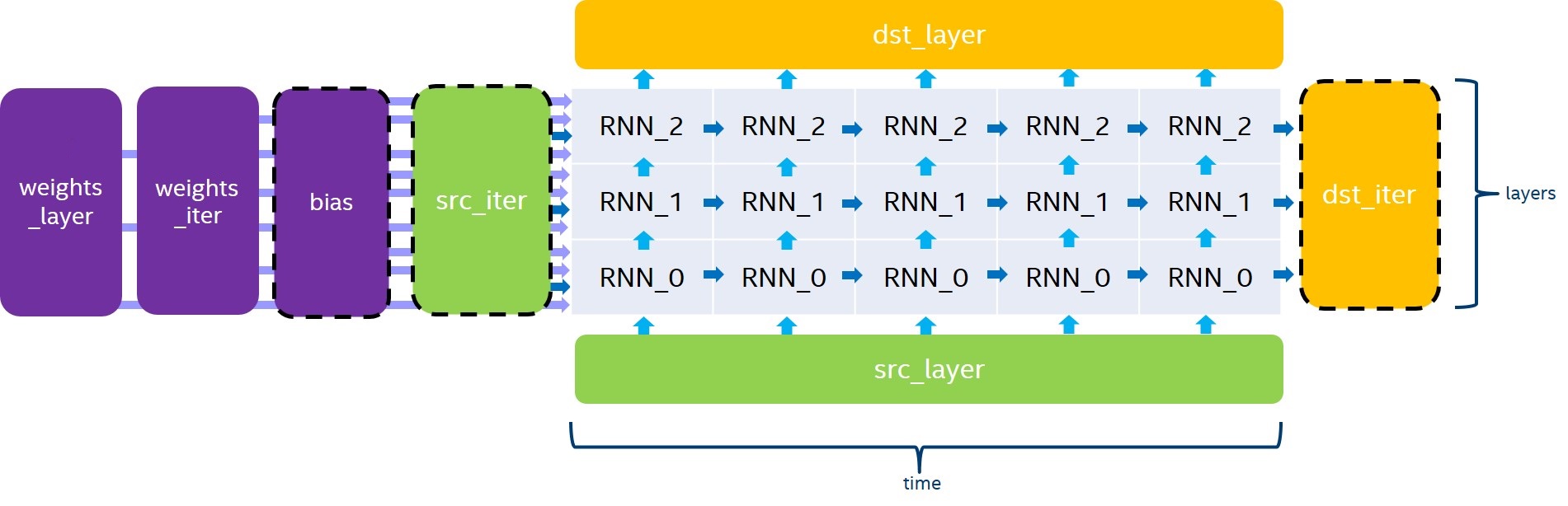
The RNN primitive computes a stack of unrolled recurrent cells, as depicted in Figure 1. \(\bias\), \(\srciter\) and \(\dstiter\) are optional parameters (the variable names follow the standard Naming Conventions). If not provided, \(\bias\) and \(\srciter\) will default to 0.
The RNN primitive supports four modes for evaluation direction:
left2right will process the input data timestamps by increasing orderright2left will process the input data timestamps by decreasing orderbidirectional_concat will process all the stacked layers from left2right and from right2left independently, and will concatenate the output in \(\dstlayer\) over the channel dimension.bidirectional_sum will process all the stacked layers from left2right and from right2left independently, and will sum the two outputs to \(\dstlayer\).Even though the RNN primitive supports passing a different number of channels for \(\srclayer\), \(\srciter\), \(\dstlayer\), and \(\dstiter\), we always require the following conditions in order for the dimension to be consistent:
bidirectional_concat direction, \(channels(\dstlayer) = 2 * channels(\dstiter)\).The general formula for the execution of a stack of unrolled recurrent cells depends on the current iteration of the previous layer ( \(h_{t,l-1}\) and \(c_{t,l-1}\)) and the previous iteration of the current layer ( \(h_{t-1, l}\)). Here is the exact equation for non-LSTM cells:
\[ \begin{align} h_{t, l} = Cell(h_{t, l-1}, h_{t-1, l}) \end{align} \]
where \(t,l\) are the indices of the timestamp and the layer of the cell being executed.
And here is the equation for LSTM cells:
\[ \begin{equation*} (h_{t, l},c_{t,l}) = Cell(h_{t, l-1}, h_{t-1, l}, c_{t-1,l}) \end{equation*} \]
where \(t,l\) are the indices of the timestamp and the layer of the cell being executed.
The RNN API provides four cell functions:
A single-gate recurrent cell initialized with dnnl::vanilla_rnn_forward::desc::desc() or dnnl::vanilla_rnn_forward::desc::desc() as in the following example.
The Vanilla RNN cell supports the ReLU, Tanh and Sigmoid activation functions. The following equations defines the mathematical operation performed by the Vanilla RNN cell for the forward pass:
\[ \begin{align} a_t &= W \cdot h_{t,l-1} + U \cdot h_{t-1, l} + B \\ h_t &= activation(a_t) \end{align} \]
A four-gate long short-term memory recurrent cell initialized with dnnl::lstm_forward::desc::desc() or dnnl::lstm_backward::desc::desc() as in the following example.
Note that for all tensors with a dimension depending on the gates number, we implicitly require the order of these gates to be i, f, \(\tilde c\), and o. The following equation gives the mathematical description of these gates and output for the forward pass:
\[ \begin{align} i_t &= \sigma(W_i \cdot h_{t,l-1} + U_i \cdot h_{t-1, l} + B_i) \\ f_t &= \sigma(W_f \cdot h_{t,l-1} + U_f \cdot h_{t-1, l} + B_f) \\ \\ \tilde c_t &= \tanh(W_{\tilde c} \cdot h_{t,l-1} + U_{\tilde c} \cdot h_{t-1, l} + B_{\tilde c}) \\ c_t &= f_t * c_{t-1} + i_t * \tilde c_t \\ \\ o_t &= \sigma(W_o \cdot h_{t,l-1} + U_o \cdot h_{t-1, l} + B_o) \\ h_t &= \tanh(c_t) * o_t \end{align} \]
where \(W_*\) are stored in \(\weightslayer\), \(U_*\) are stored in \(\weightsiter\) and \(B_*\) are stored in \(\bias\).
A four-gate long short-term memory recurrent cell with peephole initialized with dnnl::lstm_forward::desc::desc() or dnnl::lstm_backward::desc::desc() as in the following example.
Similarly to vanilla LSTM, we implicitly require the order of the gates to be i, f, \(\tilde c\), and o for all tensors with a dimension depending on the gates. For peephole weights, the gates order is i, f, o. The following equation gives the mathematical description of these gates and output for the forward pass:
\[ \begin{align} i_t &= \sigma(W_i \cdot h_{t,l-1} + U_i \cdot h_{t-1, l} + P_i \cdot c_{t-1} + B_i) \\ f_t &= \sigma(W_f \cdot h_{t,l-1} + U_f \cdot h_{t-1, l} + P_f \cdot c_{t-1} + B_f) \\ \\ \tilde c_t &= \tanh(W_{\tilde c} \cdot h_{t,l-1} + U_{\tilde c} \cdot h_{t-1, l} + B_{\tilde c}) \\ c_t &= f_t * c_{t-1} + i_t * \tilde c_t \\ \\ o_t &= \sigma(W_o \cdot h_{t,l-1} + U_o \cdot h_{t-1, l} + P_o \cdot c_t + B_o) \\ h_t &= \tanh(c_t) * o_t \end{align} \]
where \(P_*\) are stored in weights_peephole, and the other parameters are the same as in vanilla LSTM.
weights_peephole_desc passed to the operation descriptor constructor is a zero memory desciptor, the primitive will behave the same as in LSTM primitive without peephole.A four-gate long short-term memory recurrent cell with projection initialized with dnnl::lstm_forward::desc::desc() or dnnl::lstm_backward::desc::desc() as in the following example.
Similarly to vanilla LSTM, we implicitly require the order of the gates to be i, f, \(\tilde c\), and o for all tensors with a dimension depending on the gates. The following equation gives the mathematical description of these gates and output for the forward pass (for simplicity, LSTM without peephole is shown):
\[ \begin{align} i_t &= \sigma(W_i \cdot h_{t,l-1} + U_i \cdot h_{t-1,l} + B_i) \\ f_t &= \sigma(W_f \cdot h_{t,l-1} + U_f \cdot h_{t-1,l} + B_f) \\ & \\ \tilde{c}_t &= \tanh(W_{\tilde{c}} \cdot h_{t,l-1} + U_{\tilde{c}} \cdot h_{t-1,l} + B_{\tilde{c}}) \\ c_t &= f_t * c_{t-1} + i_t * \tilde{c}_t \\ & \\ o_t &= \sigma(W_o \cdot h_{t,l-1} + U_o \cdot h_{t-1,l} + B_o) \\ h_t &= R \cdot (\tanh(c_t) * o_t) \end{align} \]
where \(R\) is stored in weights_projection, and the other parameters are the same as in vanilla LSTM.
weights_projection_desc passed to the operation descriptor constructor is a zero memory desciptor, the primitive will behave the same as in LSTM primitive without projection.A three-gate gated recurrent unit cell, initialized with dnnl::gru_forward::desc::desc() or dnnl::gru_backward::desc::desc() as in the following example.
Note that for all tensors with a dimension depending on the gates number, we implicitly require the order of these gates to be u, r, and o. The following equation gives the mathematical definition of these gates.
\[ \begin{align} u_t &= \sigma(W_u \cdot h_{t,l-1} + U_u \cdot h_{t-1, l} + B_u) \\ r_t &= \sigma(W_r \cdot h_{t,l-1} + U_r \cdot h_{t-1, l} + B_r) \\ o_t &= \tanh(W_o \cdot h_{t,l-1} + U_o \cdot (r_t * h_{t-1, l}) + B_o) \\ h_t &= u_t * h_{t-1, l} + (1 - u_t) * o_t \end{align} \]
where \(W_*\) are in \(\weightslayer\), \(U_*\) are in \(\weightsiter\), and \(B_*\) are stored in \(\bias\).
A three-gate gated recurrent unit cell with linear layer applied before the reset gate, initialized with dnnl::lbr_gru_forward::desc::desc() or dnnl::lbr_gru_backward::desc::desc() as in the following example.
The following equation describes the mathematical behavior of the Linear-Before-Reset GRU cell.
\[ \begin{align} u_t &= \sigma(W_u \cdot h_{t,l-1} + U_u \cdot h_{t-1, l} + B_u) \\ r_t &= \sigma(W_r \cdot h_{t,l-1} + U_r \cdot h_{t-1, l} + B_r) \\ o_t &= \tanh(W_o \cdot h_{t,l-1} + r_t *(U_o \cdot h_{t-1, l} + B_{u'}) + B_o) \\ h_t &= u_t * h_{t-1, l} + (1 - u_t) * o_t \end{align} \]
Note that for all tensors with a dimension depending on the gates number, except the bias, we implicitly require the order of these gates to be u, r, and o. For the \(\bias\) tensor, we implicitly require the order of the gates to be u, r, o, and ‘u’`.
When using the RNN API for training, the forward pass should use the forward_training propagation kind, and a workspace should be passed to both the forward pass and the backward pass. Note that after executing the backward pass, the workspace is no more valid and should be populated once again by another forward pass.
When executed, the inputs and outputs should be mapped to an execution argument index as specified by the following table.
| Primitive input/output | Execution argument index |
|---|---|
| \(\srclayer\) | DNNL_ARG_SRC_LAYER |
| \(\srciter\) | DNNL_ARG_SRC_ITER |
| \(\srciterc\) | DNNL_ARG_SRC_ITER_C |
| \(\weightslayer\) | DNNL_ARG_WEIGHTS_LAYER |
| \(\weightsiter\) | DNNL_ARG_WEIGHTS_ITER |
| \(\weightspeephole\) | DNNL_ARG_WEIGHTS_PEEPHOLE |
| \(\weightsprojection\) | DNNL_ARG_WEIGHTS_PROJECTION |
| \(\bias\) | DNNL_ARG_BIAS |
| \(\dstlayer\) | DNNL_ARG_DST_LAYER |
| \(\dstiter\) | DNNL_ARG_DST_ITER |
| \(\dstiterc\) | DNNL_ARG_DST_ITER_C |
| \(\workspace\) | DNNL_WORKSPACE |
| \(\diffsrclayer\) | DNNL_ARG_DIFF_SRC_LAYER |
| \(\diffsrciter\) | DNNL_ARG_DIFF_SRC_ITER |
| \(\diffsrciterc\) | DNNL_ARG_DIFF_SRC_ITER_C |
| \(\diffweightslayer\) | DNNL_ARG_DIFF_WEIGHTS_LAYER |
| \(\diffweightsiter\) | DNNL_ARG_DIFF_WEIGHTS_ITER |
| \(\diffweightspeephole\) | DNNL_ARG_DIFF_WEIGHTS_PEEPHOLE |
| \(\diffweightsprojection\) | DNNL_ARG_DIFF_WEIGHTS_PROJECTION |
| \(\diffbias\) | DNNL_ARG_DIFF_BIAS |
| \(\diffdstlayer\) | DNNL_ARG_DIFF_DST_LAYER |
| \(\diffdstiter\) | DNNL_ARG_DIFF_DST_ITER |
| \(\diffdstiterc\) | DNNL_ARG_DIFF_DST_ITER_C |
The following table lists the combination of data types supported by the RNN primitive for each input and output memory object.
| Propagation | Cell Function | Input data | Recurrent data (1) | Weights | Bias | Output Data |
|---|---|---|---|---|---|---|
| Forward / Backward | All | f32 | f32 | f32 | f32 | f32 |
| Forward / Backward (2) | All (3) | bf16 | bf16 | bf16 | f32 | bf16 |
| Forward | All (3) | f16 | f16 | f16 | f16 | f16 |
| Forward inference | Vanilla LSTM, LSTMP and GRU | u8 | u8 | s8 | f32 | u8, f32 |
(1) With LSTM and Peephole LSTM cells, the cell state datatype is always f32.
(2) In backward propagation, all diff_* tensors are in f32.
(3) Projection LSTM is not supported.
In the oneDNN programming model, the RNN primitive is one of a few that support the placeholder memory format dnnl::memory::format_tag::any (shortened to any from now on) and can define data and weight memory objects format based on the primitive parameters.
The following table summarizes the data layouts supported by the RNN primitive.
| Propagation | Input/Output Data | Recurrent Data | Layer and Iteration Weights | Peephole Weights and Bias | Projection LSTM Weights ----— |
|---|---|---|---|---|---|
| Forward / Backward | any | any | any | ldgo | any |
| Forward | ntc, tnc | ldnc | ldigo | ldgo | ldio |
| Backward | ntc, tnc | ldnc | ldgoi | ldgo | ldoi |
While an RNN primitive can be created with memory formats specified explicitly, the performance is likely to be sub-optimal. When using any it is necessary to first create an RNN primitive descriptor and then query it for the actual data and weight memory objects formats.
Currently post-ops and attributes are only used by the int8 variants of LSTM and GRU. See the markdown RNN int8 inference example for more details on how to use and set these quantization parameters.
| Engine | Name | Com |
|---|---|---|
| CPU/GPU | LSTM RNN Primitive Example | This C++ API example demonstrates how to create and execute an LSTM RNN primitive in forward training propagation mode. Key optimizations included in this example:
|

