Introduction
Most of the computations are about data: analyzing data, adjusting data, reading and storing data, generating data... DNN domain is no exception. Images, weights/filters, sound, and text require efficient representation in computer memory to perform operations fast and in the most convenient way.
This article is devoted to data format – one form of data representation that describes how multidimensional arrays (nD) are stored in linear (1D) memory address space and why this is important for Intel(R) Math Kernel Library for Deep Neural Networks (Intel(R) MKL-DNN).
Note: for the purpose of this article data format and layout are used interchangeably.
Nomenclature used
- Channels mean the same as feature maps
- Upper-case letters denote the dimensions (e.g.
N) - Lower-case letters denote the index (e.g.
n, where0 <= n < N) The notation for the activations:
batch N, channels C, depth D, height H, width W
The notation for the weights:
groups G, output channels O, input channels I, depth D, height H, width W
Data formats
Let's first focus on data formats for activations (images).
Activations consist of channels (aka feature maps) and a spatial domain, 1D, 2D or 3D. Spatial domain together with channels form an image. During the training phase images are typically grouped together in batches. Even if there is only one image, we would still assume there is a batch with batch size equal to 1. Hence, the overall dimensionality of activations is 4D (N, C, H, and W) or 5D (N, C, D, H, and W).
In this article for the sake of simplicity we will use 2D spatial only.
Plain data formats
It would be simpler to start with an example.
Consider 4D activations with batch equals 2, 16 channels, and 5 x 4 spatial domain. Logical representation is given on the picture below.
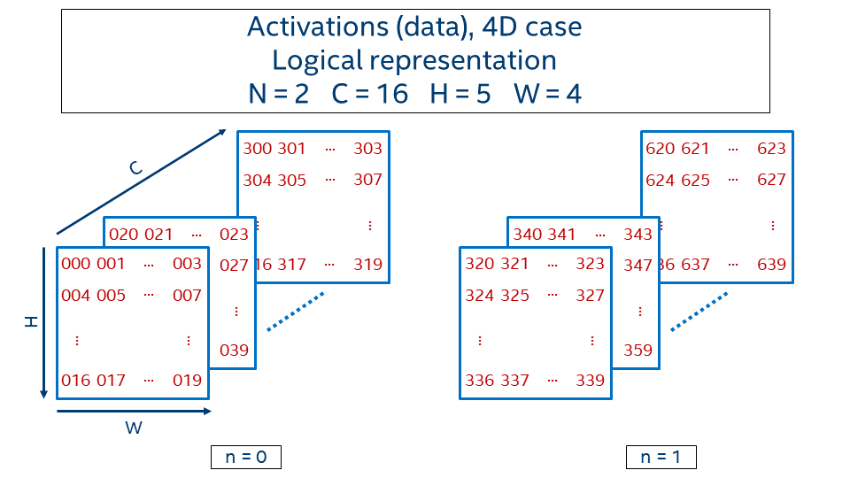
The value at the position (n, c, h, w) is generated with the following formula:
In order to define how data in this 4D-tensor is laid out in memory we need to define how to map it to a 1D tensor via an offset function that takes logical index (n, c, h, w) as an input and returns an address displacement to where the value is located:
NCHW
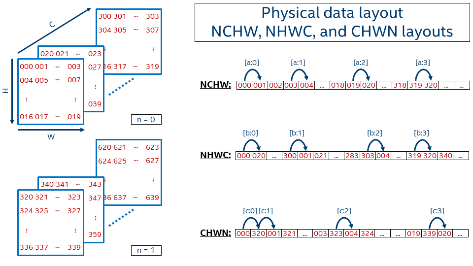
Let's describe the order in which the tensor values are laid out in memory for one the very popular format NCHW. The [a:?] marks refer to the jumps shown in the picture below that shows the 1D representation of an NCHW tensor in memory.
[a:0]First within a line, from left to right[a:1]Then line by line from top to bottom[a:2]Then go from one plane to another (in depth)[a:3]And finally switch from one image in a batch (n = 0) to another (n = 1)
Then the offset function is:
We use nchw here to denote that w is the inner-most dimension, meaning that two elements adjacent in memory would share the same indices of n, c, and h, and their index of w would be different by 1. This is of course true only for non-border elements. On the contrary n is the outermost dimension here, meaning that if you need to take the same pixel (c, h, w) but on the next image you have to jump over the whole image size C*H*W.
This data format is called NCHW and used by default in BVLC* Caffe. TensorFlow* also supports this data format.
Note: It is just a coincidence that
offset_nchw()is the same asvalue()in this example.
One can create memory with NCHW data layout using mkldnn_nchw of the enum type mkldnn_memory_format_t defined in mkldnn_types.h for C API and mkldnn::memory::nchw defined in mkldnn.hpp for C++ API.
NHWC
Another quite popular data format is NHWC and it uses the following offset function:
In this case the inner-most dimension is channels ([b:0]) that is followed by width ([b:1]), height ([b:2]), and finally batch ([b:3]).
For a single image (N = 1), this format is very similar to how BMP-file format works, where the image is kept pixel by pixel and every pixel contains all required information about colors (for instance 3 channels for 24bit BMP).
NHWC data format is the default one for TensorFlow.
This layout corresponds to mkldnn_nhwc or mkldnn::memory::nhwc.
CHWN
The last example here for the plain data layout is CHWN which is used by Neon. This layout might be very interesting from a vectorization perspective if an appropriate batch size is used, but on the other hand users cannot always have good batch size (e.g. in case of real-time inference batch is typically 1).
The dimensions order is (from inner-most to outer-most): batch ([c:0]), width ([c:1]), height ([c:2]), channels ([c:3]).
The offset function for CHWN format is defined as:
This layout corresponds to mkldnn_chwn or mkldnn::memory::chwn.
Relevant reading
TensorFlow Doc. Shapes and Layout
Generalization of the plain data layout
Strides
In the previous examples the data was kept packed or in dense form, meaning pixels follow one another. Sometimes it might be necessary to not keep data contiguous in memory. For instance some might need to work with sub-tensor within a bigger tensor. Sometimes it might be beneficial to artificially make the data disjoint, like in case of GEMM with non-trivial leading dimension to get better performance (see Tips 6).
The following picture shows simplified case for 2D matrix of size rows x columns kept in row-major format where rows have some non-trivial (i.e. not equal to the number of columns) stride.
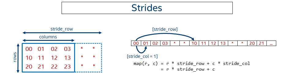
In this case the general offset function looks like:
Note, then NCHW, NHWC, and CHWN formats are just special cases of the format with strides. For example for NCHW we have:
Intel MKL-DNN supports strides via blocking structure. The pseudo code is:
In particular whenever a user creates memory with mkldnn_nchw format MKL-DNN computes the strides and fills the structure on behalf of the user. That can be done manually though.
Blocked layout
Plain layouts give great flexibility and are very convenient for use. That's why most of the frameworks and applications use either NCHW or NHWC layouts. However depending on the operation that is performed on data it might turn out that those layouts are sub-optimal from performance perspective.
In order to achieve better vectorization and cache re-usage Intel MKL-DNN introduces blocked layout that splits one or several dimensions into the blocks of fixed size. The most popular Intel MKL-DNN data format is nChw16c on AVX512+ systems and nChw8c on SSE4.2+ systems. As one might guess from the name the only dimension that is blocked is channels and the block size is either 16 in the former case or 8 in the later case.
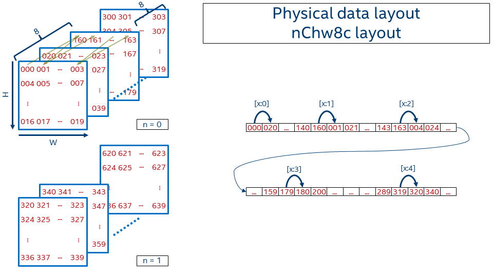
Precisely, the offset function for nChw8c is:
Note that blocks of 8 channels are kept contiguously in memory. Pixel by pixel the spatial domain is covered. Then next slice covers subsequent 8 channels (i.e. moving from c=0..7 to c=8..15). Once all channel blocks are covered the next image in the batch appears.
Note: we use lower- and uppercase letters in the formats to distinguish between the blocks (e.g. 8c) and the remaining co-dimension (C = channels / 8).
The reason behind the format choice can be found in this paper.
Intel MKL-DNN describes this type of memory via blocking structure as well. The pseudo code is:
What if channels are not multiple of 8 (or 16)?
Blocking data layout gives significant performance improvement for the convolutions, but what to do when the number of channels is not multiple of the block size, say 17 channels for nChw8c format?
Well one of the possible ways to handle that would be to use blocked layout for as many channels as possible by rounding them down to a number that is a multiple of the block size (in this case 16 = 17 / 8 * 8) and process the tail somehow. However that would lead to introduction of very special tail processing code into many Intel MKL-DNN kernels.
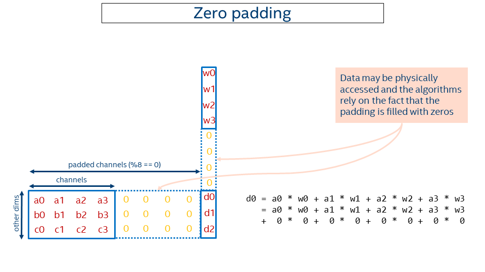
So we came up with another solution using zero-padding. The idea is to round the channels up to make them multiples of the block size and pad created tail with zeros (in the example above 24 = div_up(17, 8) * 8). Then primitives like convolutions might work with rounded-up number of channels instead of the original ones and compute the correct result (adding zeros doesn't change the result).
That allows supporting arbitrary number of channels with almost no changes to the kernels. The price would be some extra computations on those zeros, but this is either negligible or the performance with overheads is still higher than the performance with plain data layout.
The picture below depicts the idea. Note that some extra computations happen while computing d0, but that does not affect the result.
The feature is supported starting with Intel MKL-DNN v0.15. So far the support is limited by f32 data type and on the AVX512+ systems. We plan to extend the implementations for other cases as well.
Some pitfalls of the given approach:
- To keep padded data are zeros invariant mkldnn_memory_set_data_handle() and mkldnn::memory::set_data_handle() physically put zeros whenever user attaches a pointer to a memory that uses zero padding. That might affect performance if too many unnecessary calls to these functions are made. We might consider extending our API in future to allow attaching pointers without subsequent initialization with zeros, if user can guarantee the padding is already filled correctly
- Memory size required to keep the data cannot be computed by the formula
sizeof(data_type) * N * C * H * Wanymore. Actual size should always be queried via mkldnn_memory_primitive_desc_get_size() in C and mkldnn::memory::primitive_desc::get_size() in C++ - Element-wise operations that are implemented in user's code and directly operate on Intel MKL-DNN blocked layout like that: are not safe if the data is padded with zeros and thefor (int e = 0; e < phys_size; ++e)x[e] = eltwise_op(x[e])
eltwise_op(0) != 0
Relevant Intel MKL-DNN code: